
Using DuckDB-WASM for in-browser Data Engineering
Introduction#
DuckDB, the in-process DBMS specialized in OLAP workloads, had a very rapid growth during the last year, both in functionality, but also popularity amongst its users, but also with developers that contribute many projects to the Open Source DuckDB ecosystem.
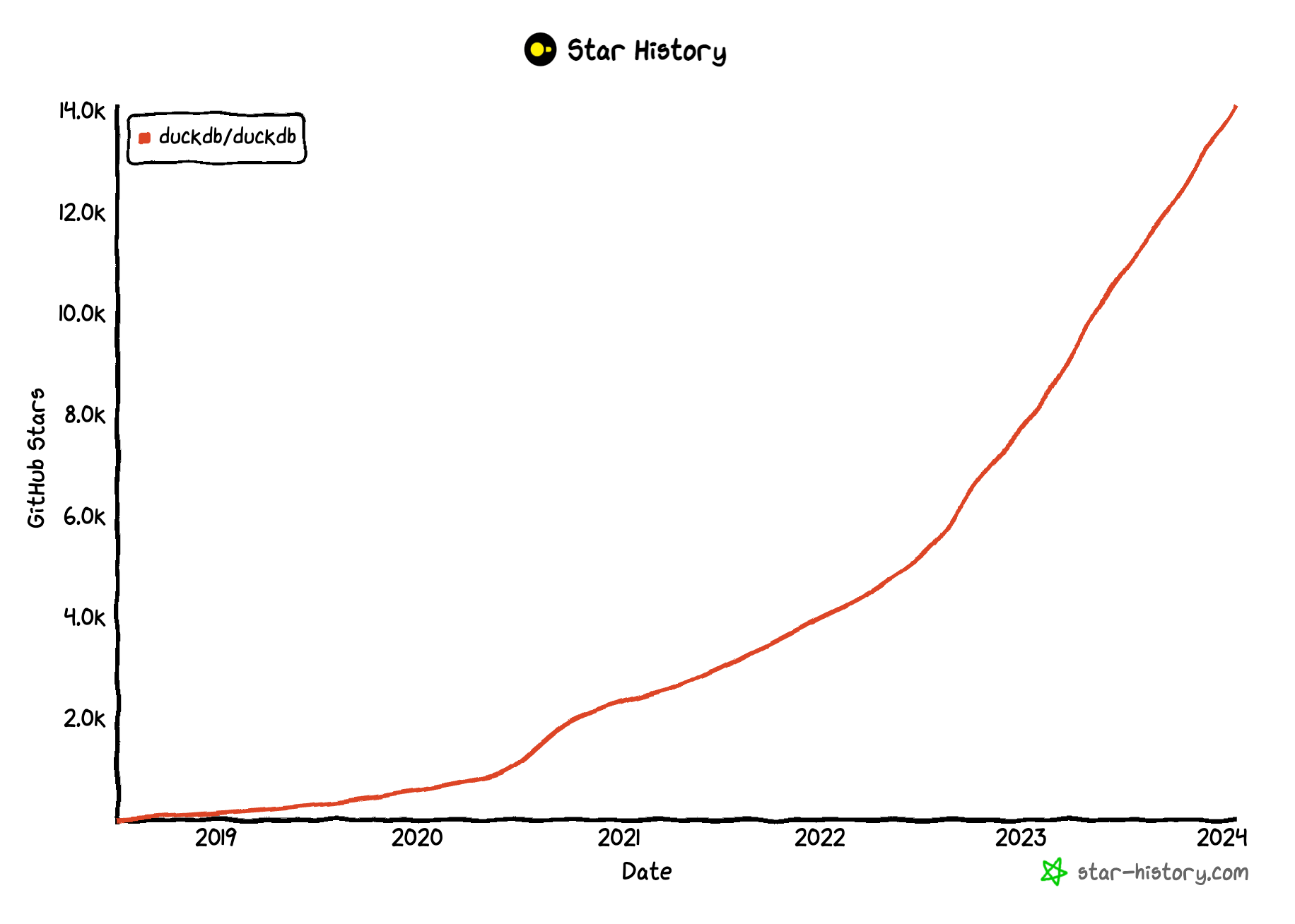
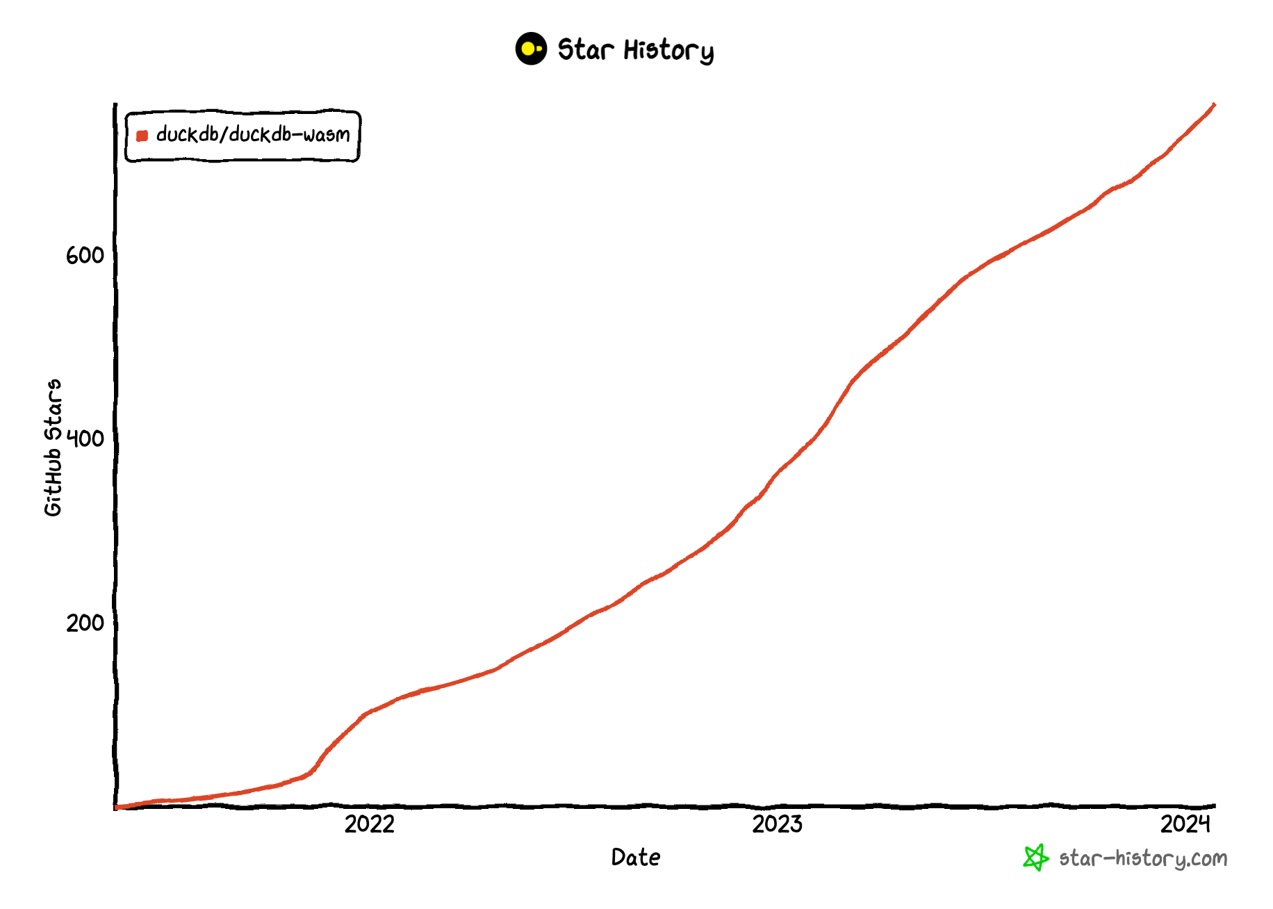
DuckDB cannot “only” be run on a variety of Operating Systems and Architectures, there’s also a DuckDB-WASM version, that allows running DuckDB in a browser. This opens up some very interesting use cases, and is also gaining a lot of traction in the last 12 months.
Use Case: Building a SQL Workbench with DuckDB-WASM#
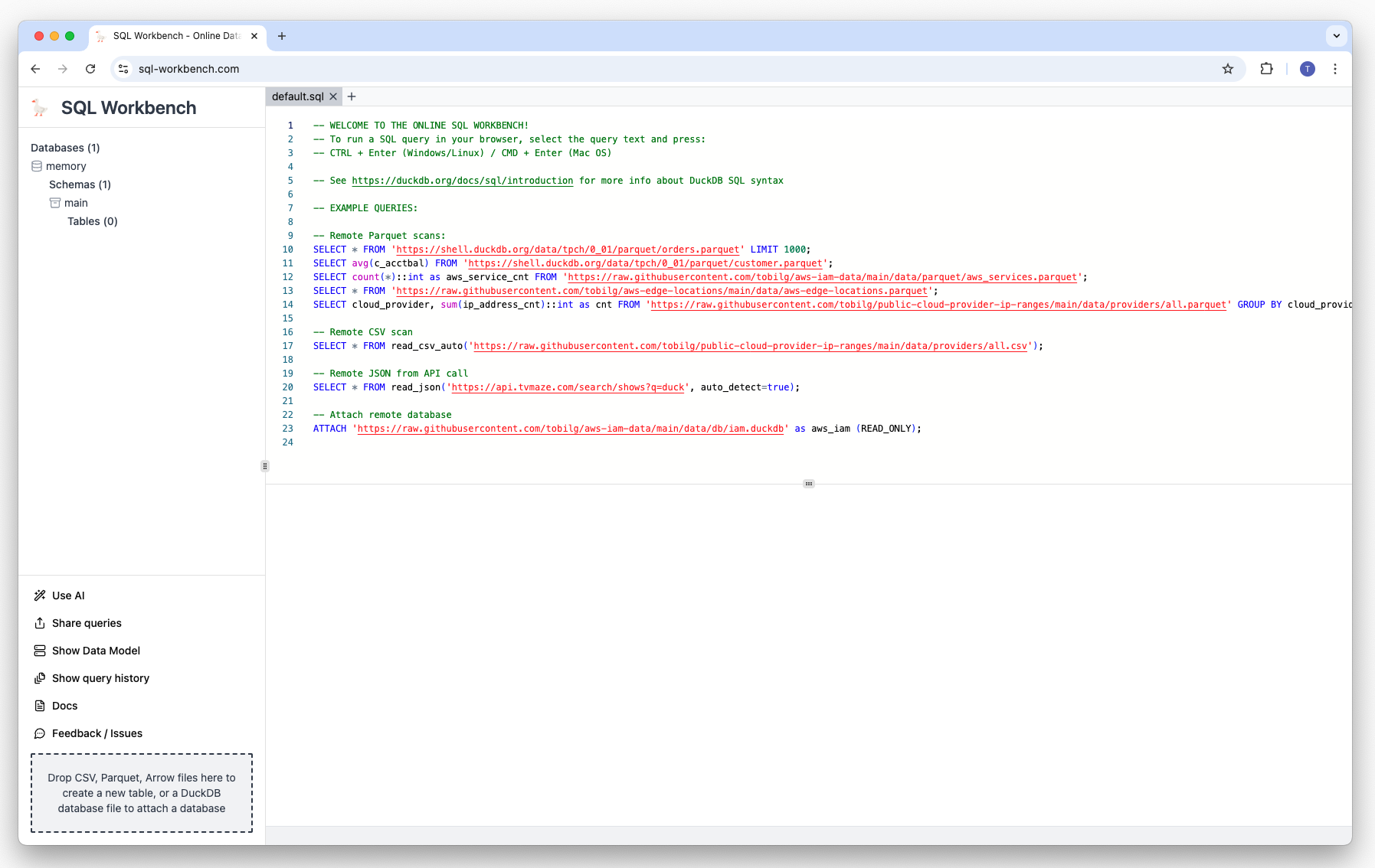
One of the first things that came to my mind once I learned about the existence of DuckDB-WASM was that it could be used to create an online SQL Workbench, where people could interactively run queries, show their results, but also visualize them. DuckDB-WASM sits at its core, providing the storage layer, query engine and many things more…
You can find the project at
It’s built with the following core technologies / frameworks:
It’s hosted as a static website export / single page application on AWS using
-
CloudFront as CDN
-
S3 as file hosting service
-
ACM for managing certificates
-
Route53 for DNS
If you’re interested in the hosting setup, you can have a look at https://github.com/tobilg/serverless-aws-static-websites which can deploy such static websites on AWS via IaC with minimum effort.
Using the SQL Workbench#
There are many possibilities how you can use the SQL Workbench, some are described below
Overview#
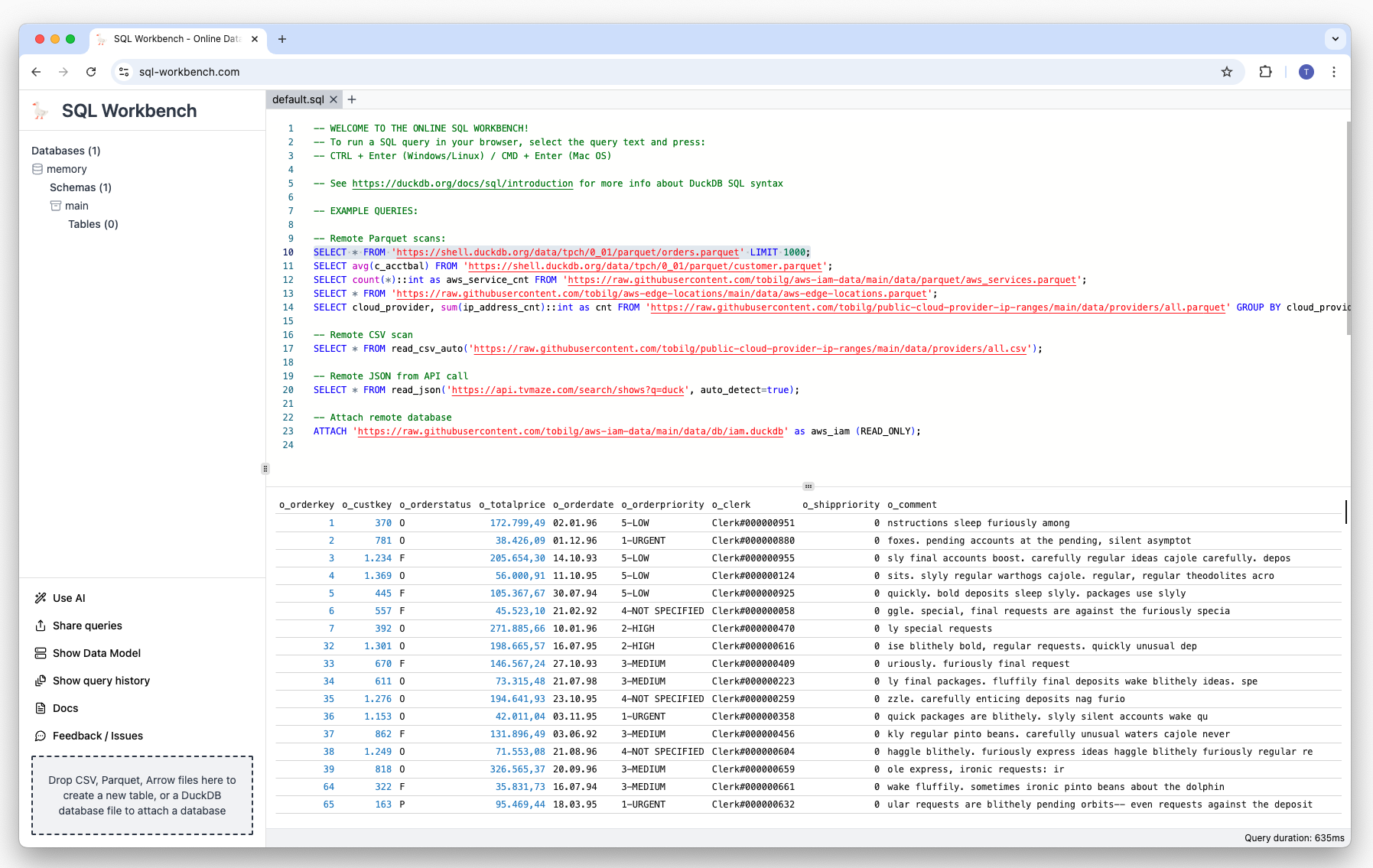
When you open sql-workbench.com for the first time, you can see that the workbench is divided in three different areas:
-
On the left, there’s the “Local Tables” area, that will display the created tables of you ran queries such as
CREATE TABLE names (name VARCHAR), or used the drag-and-drop area on the lower left corner to drop any CSV, Parquet or Arrow file on it (details see below). -
The upper main editor area is the SQL editor, where you can type your SQL queries. You’re already presented with some example queries for different types of data once the page is loaded.
-
The lower main result area where the results of the ran queries will be shown, or alternatively, the visualizations of these results.
Running SQL queries#
To run your first query, select the first line of SQL, either with your keyboard or with your mouse, and press the key combination CMD + Enter of you’re on a Mac, or Ctrl + Enter if you’re on a Windows or Linux machine.
The result of the query that was executed can then be found in the lower main area as a table:
Running multiple queries#
You can also run multiple queries sequentially, e.g. to create a table, insert some records, and display the results:
CREATE TABLE first_names (name VARCHAR, birth_cnt integer);

INSERT INTO first_names (name, birth_cnt) VALUES ('Liam', 20456);
INSERT INTO first_names (name, birth_cnt) VALUES ('Noah', 18621);
INSERT INTO first_names (name, birth_cnt) VALUES ('Oliver', 15076);
INSERT INTO first_names (name, birth_cnt) VALUES ('James', 12028);
INSERT INTO first_names (name, birth_cnt) VALUES ('Elijah', 11979);
INSERT INTO first_names (name, birth_cnt) VALUES ('William', 11282);
INSERT INTO first_names (name, birth_cnt) VALUES ('Henry', 11221);
INSERT INTO first_names (name, birth_cnt) VALUES ('Lucas', 10909);
INSERT INTO first_names (name, birth_cnt) VALUES ('Benjamin', 10842);
INSERT INTO first_names (name, birth_cnt) VALUES ('Theodore', 10754);

SELECT * FROM first_names;
When you copy & paste the above SQLs, select them and run them, the result looks like this:
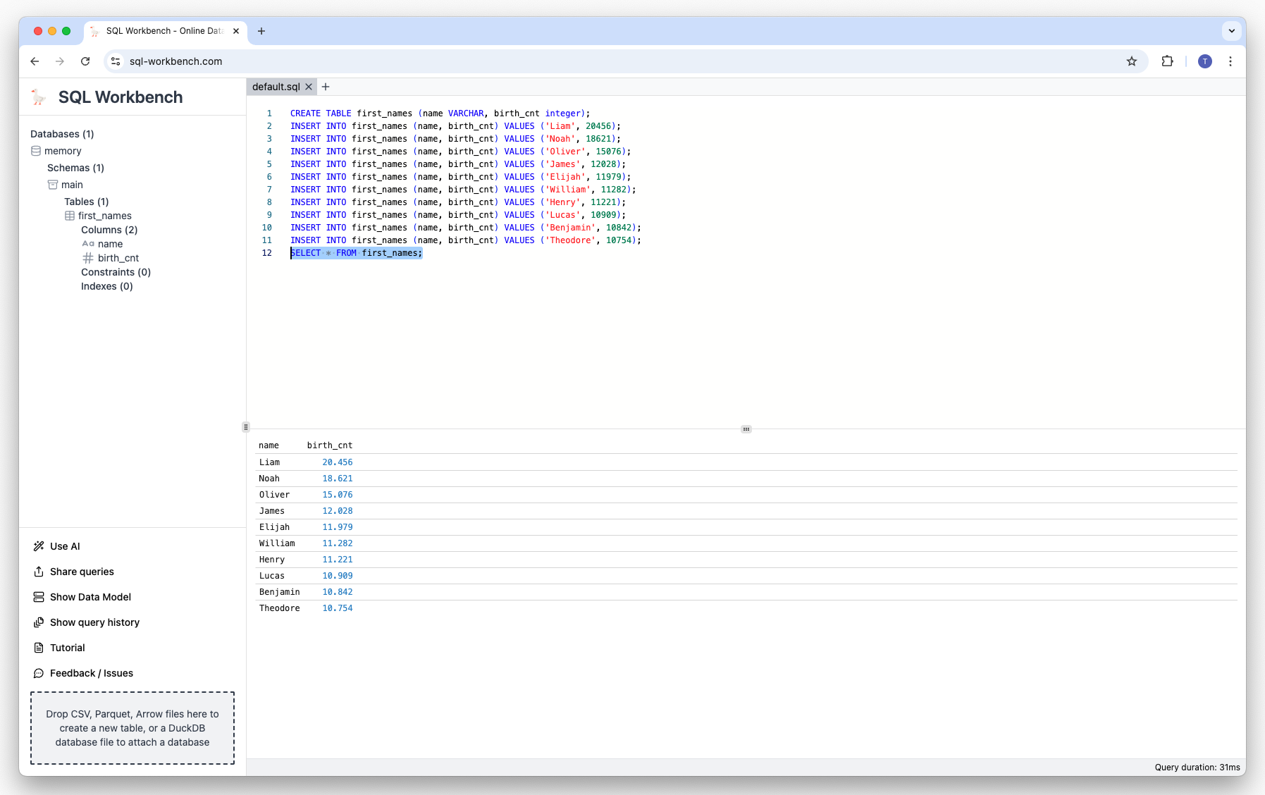
You can see on the left-hand side the newly created table first_names, that can be reused for other queries without having to reload the data again.
If you want to open a new SQL Workbench and directly run the above query, please click on the image below:

Querying data you have on your machine#
To try this, you can for example download a list of AWS Services as a CSV from
https://raw.githubusercontent.com/tobilg/aws-iam-data/main/data/csv/aws_services.csv
This file has four columns, service_id, name, prefix and reference_url. Once you downloaded the file, you can simply drag-and-drop from the folder you downloaded it to to the area in the lower left corner of the SQL Workbench:
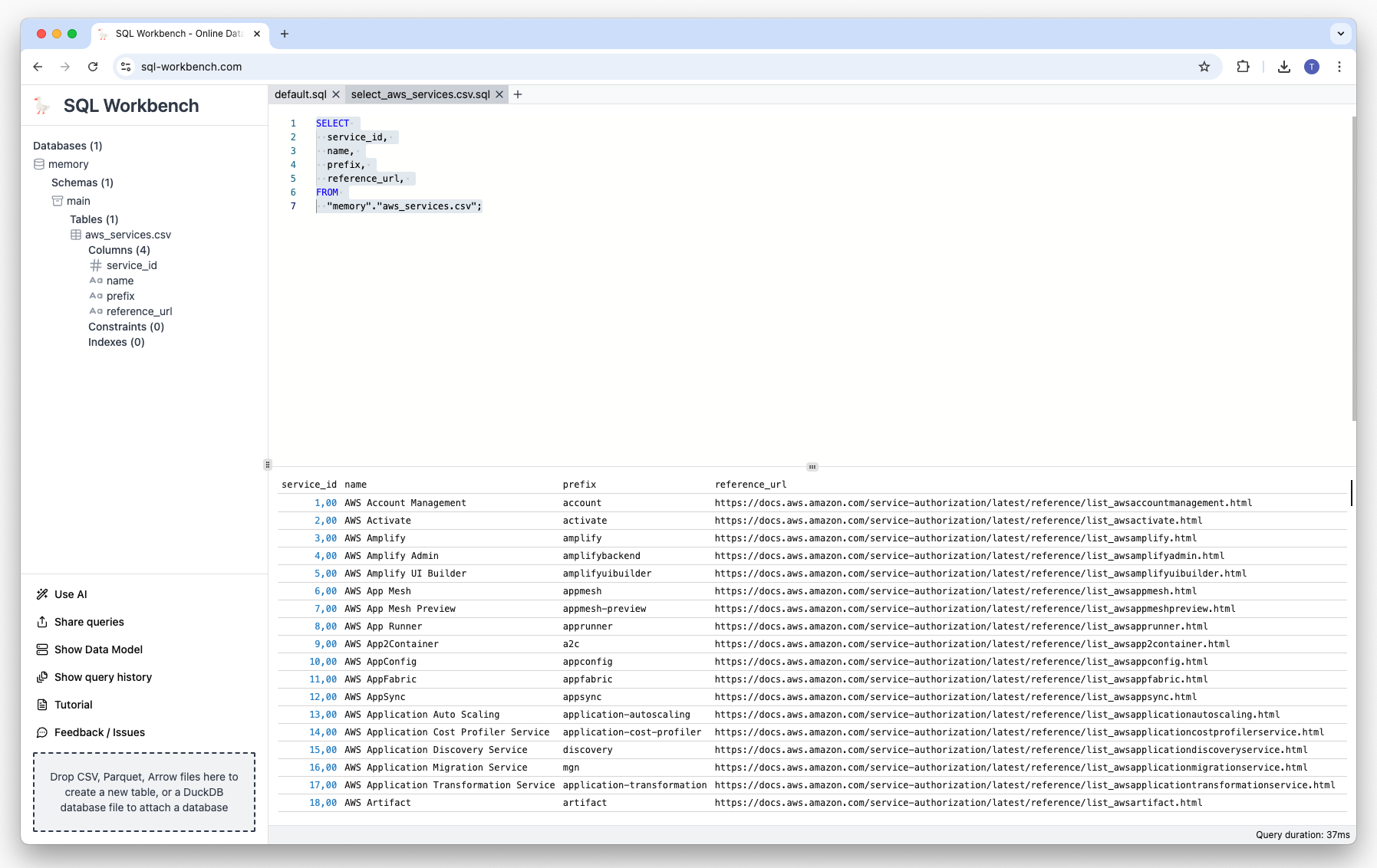
A table called aws_services.csv has now been automatically created, which you can query via SQLs, for example:
SELECT name, prefix from 'aws_services.csv';If you want to open a new SQL Workbench and directly run the above query, please click on the image below:
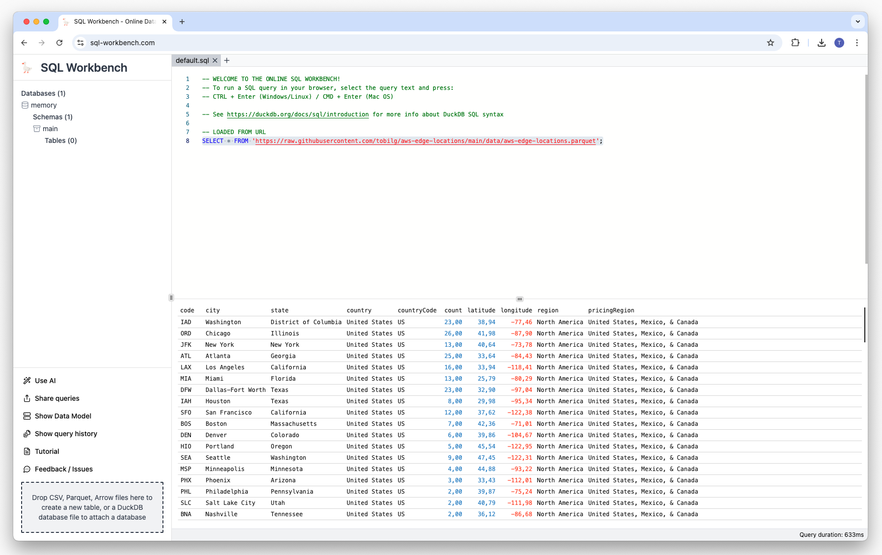
Querying and visualizing remote data#
DuckDB-WASM supports the loading of compatible data in different formats (e.g. CSV, Parquet or Arrow) from remote http(s) sources. Other data formats that can be used include JSON, but this requires the loading of so-called DuckDB extensions.
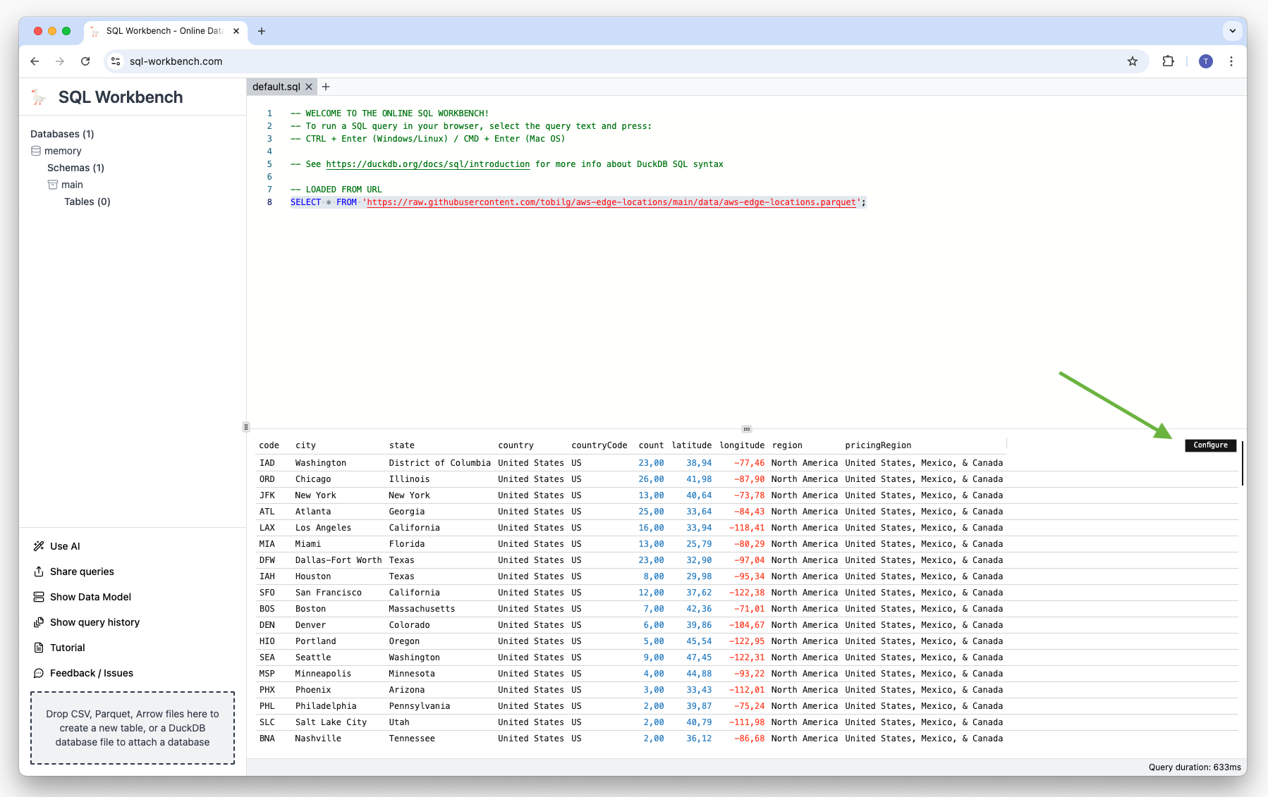
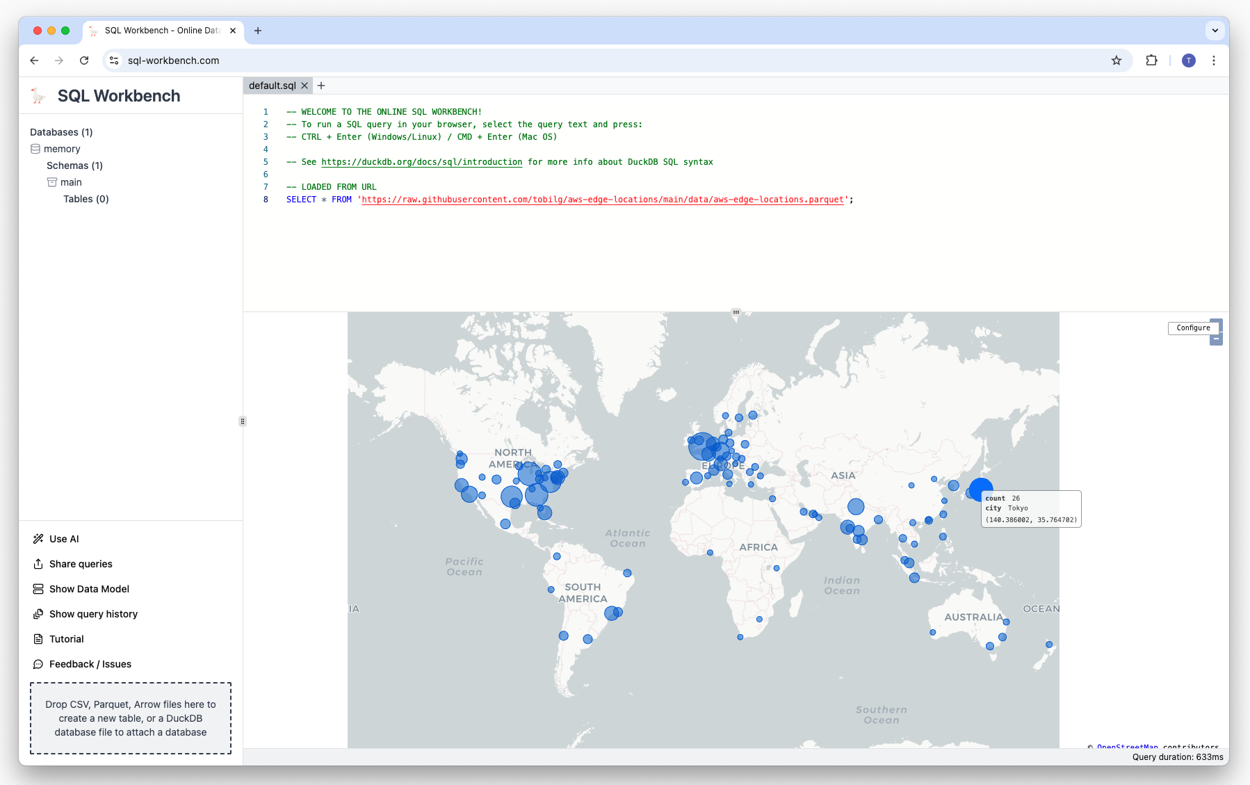
In this example, we will use data about AWS CloudFront Edge Locations, that is available at tobilg/aws-edge-locations with this query:
SELECT * FROM 'https://raw.githubusercontent.com/tobilg/aws-edge-locations/main/data/aws-edge-locations.parquet';The result will look like this:
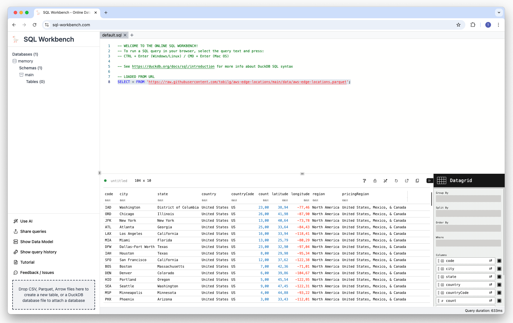
We now want to create a bar chart of the data, showing the number of Edge Locations by country and city. This can be done by hovering over the result table, and clicking on the small “configure” button that looks like a wrench which subsequently appears on the upper right corner of the table:
You then see the overview of the available columns, and the current visualization type (Datagrid)
To get an overview of the possible visualization types click on the Datagrid icon:
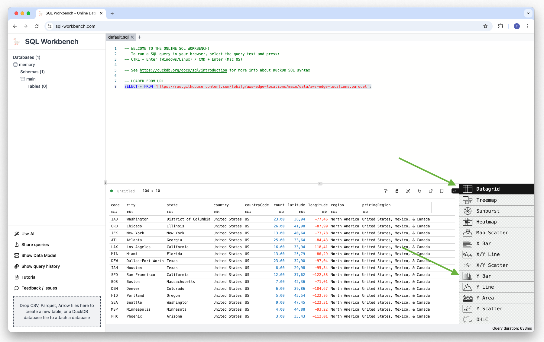
Then select “Y Bar”. This will give you an initial bar char:
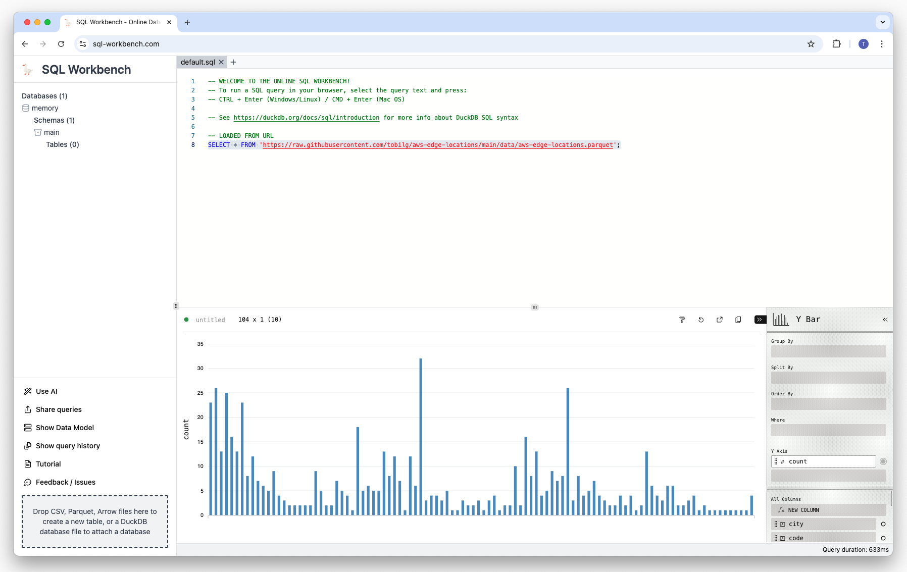
But as we want to display the count of Edge Locations by country and city, we need to drag-and-drop the columns country and city to the “Group By” area:
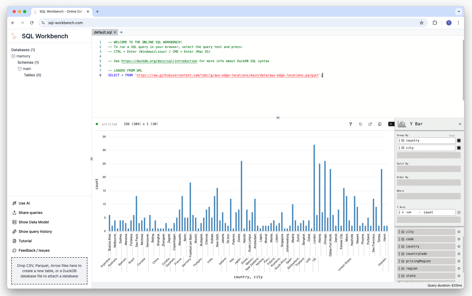
We can now close the configuration menu to see the chart in it’s full size:
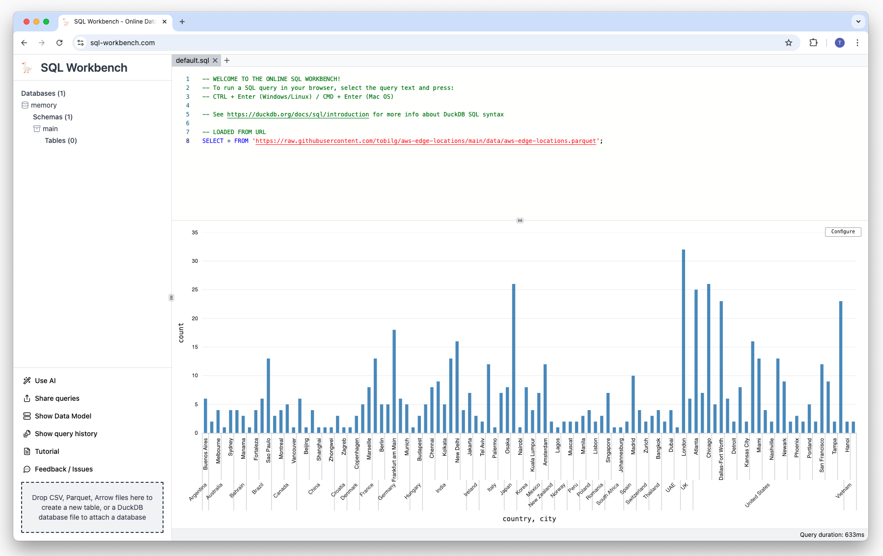
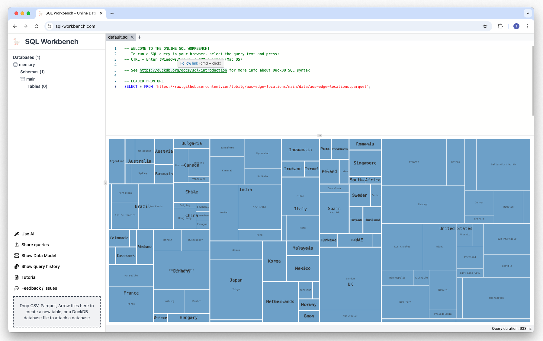
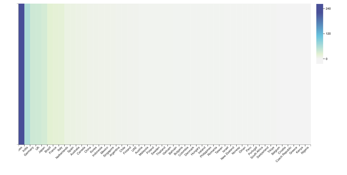
There are many other visualization types from which you can choose from, such as Treemaps and Sunbursts, as well as Map Scatters:
Exporting visualizations and data#
You can also export the visualizations, as well as the data. Just click on “Export” and type in a “Save as” name, and select the output format you want to download:
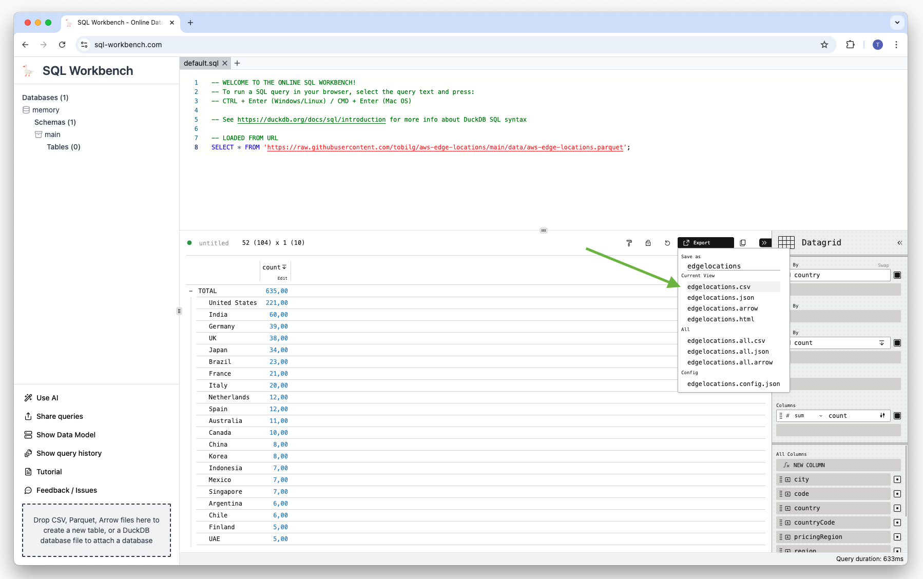
The data can be downloaded as CSV, JSON or Arrow file. Here’s the CSV example:
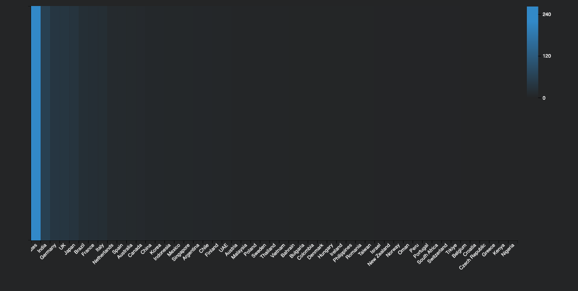
"country (Group by 1)","count"
,517
"Argentina",3
"Australia",10
"Austria",3
"Bahrain",2
"Belgium",1
"Brazil",21
"Bulgaria",3
"Canada",8
"Chile",6
"China",8
"Colombia",3
"Croatia",1
"Czech Republic",1
"Denmark",3
"Finland",4
"France",17
"Germany",37
"Greece",1
"Hungary",1
"India",48
"Indonesia",5
"Ireland",2
"Israel",2
"Italy",16
"Japan",27
"Kenya",1
"Korea",8
"Malaysia",2
"Mexico",4
"Netherlands",5
"New Zealand",2
"Nigeria",1
"Norway",2
"Oman",1
"Peru",2
"Philippines",2
"Poland",5
"Portugal",1
"Romania",1
"Singapore",7
"South Africa",2
"Spain",12
"Sweden",4
"Switzerland",2
"Taiwan",3
"Thailand",2
"UAE",4
"UK",30
"United States",179
"Vietnam",2
And here’s the exported PNG:
Exporting the HTML version will give you an interactive graph with hovering etc. Furthermore, you can also change the theme for the different visualizations:
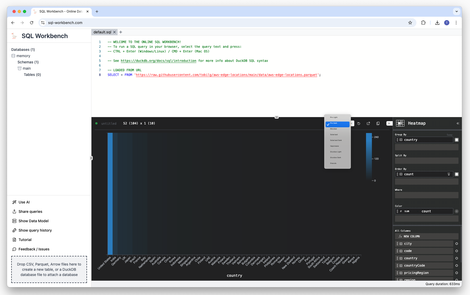
This is also reflected in the exported graphs:
Using the schema browser#
The schema browser can be found on the left-hand side. It’s automatically updated after each executed query, so that all schema operations can be captured. On table-level, the columns, constraints and indexes are shown:
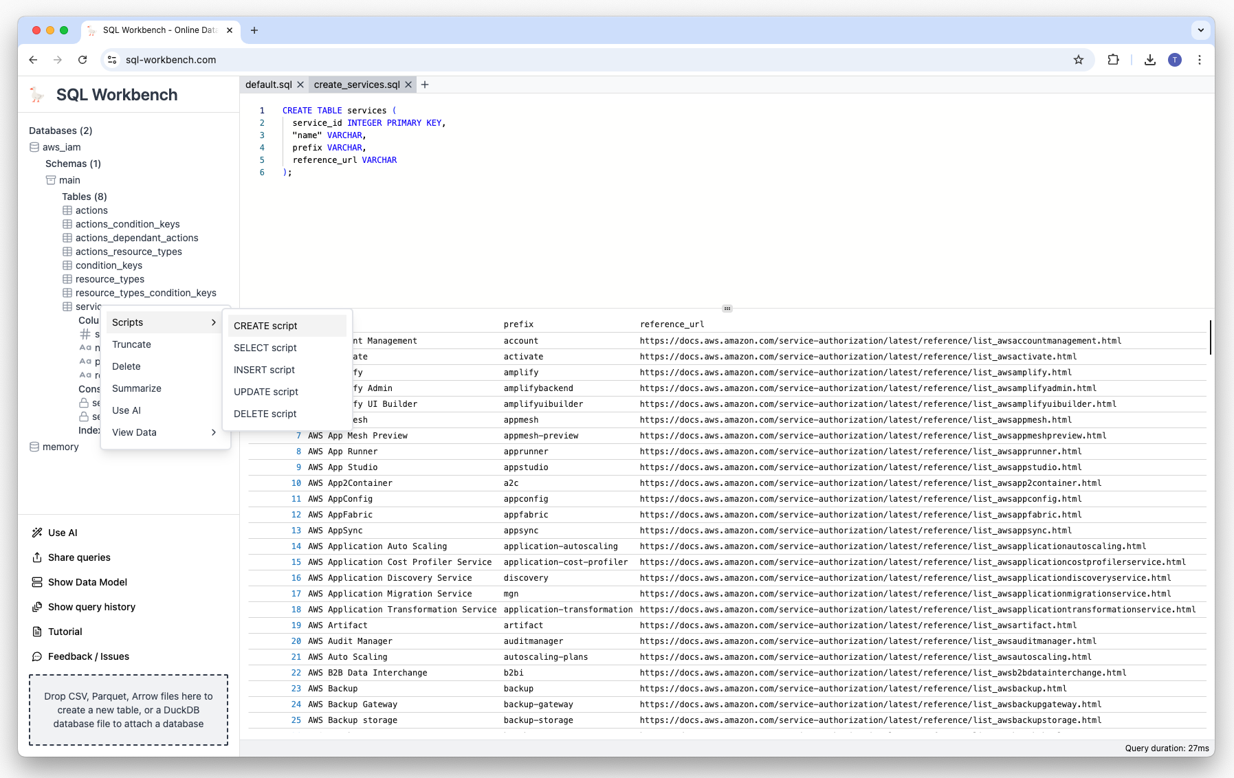
If you right-click on a table name, a context menu is shown that has different options:
-
Generating scripts based on the table definition
-
Truncating, deleting or summarizing the table
-
Viewing table data (all records, first 10 and first 100)
Once clicked, those menu items will create a new tab (see below), and generate and execute the appropriate SQL statements:
Using query tabs#
Another new feature is the possibility to have multiple query tabs. Those are either automatically created by context menu actions, or the user that clicks on the plus icon:
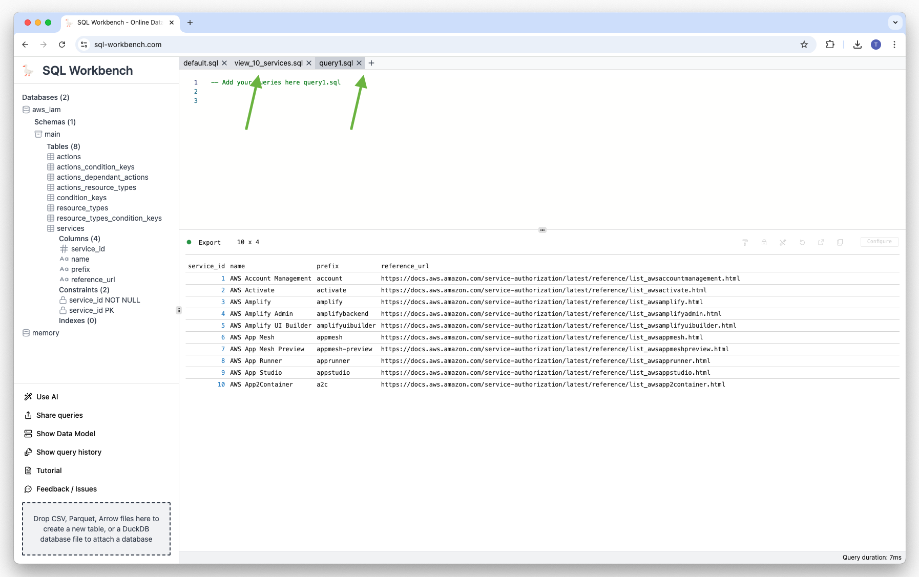
Each tab can be closed by clicking on the “x” icon next to the tab name.
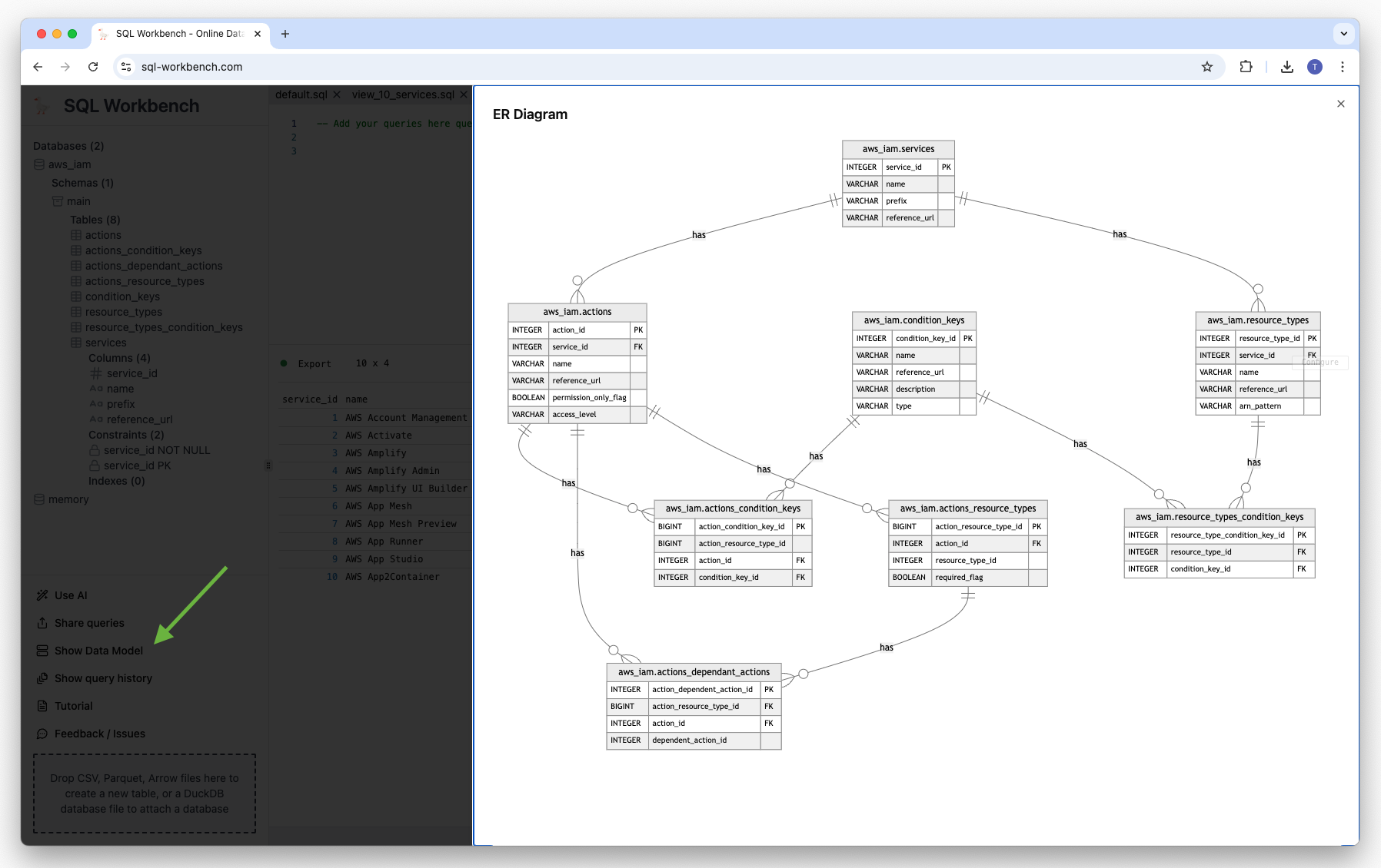
Generating data models#
If users have created some tables, it’s then possible to create a data model from the schema metadata. If the tables also have foreign key relationships, those are also shown in the diagram. Just click on the “Data Model” menu entry on the lower left corner.
Under the hood, this feature generates Mermaid Entity Relationship Diagram code, that is dynamically rendered as a graph.
Using the query history#
Each query that is issued in the current version of the SQL Workbench is recorded for the so-called query history. It can be accessed by clicking on the “Query History” menu entry in the lower left corner. Once clicked, there’s an overlay on the right-hand side with the list of the issued queries.
The newest queries can be found on top of the list, and with each query listed, there’s also an indication when the query was run, and how long it took to execute.
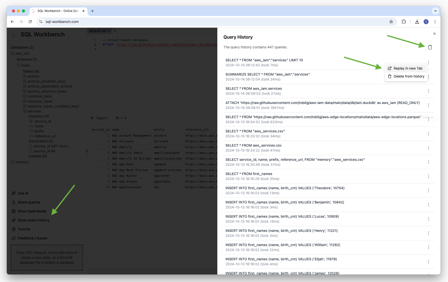
With the trash icon in the top-right corner, the complete query history can be truncated. Also, single query history entries can be deleted, as well as specific queries can be re-run in a new tab by clicking “Replay query” in the menu that’s present for each query history entry.
Example Data Engineering pipeline#
Dataset & Goals#
A well-known dataset is the NYC TLC Trip Record dataset. It can be found freely available on the website of NYC Taxi and Limousine Commission website. It also comes with some explanations and additional lookup data. In this example, we focus on the yellow taxi data.
The goal of this example pipeline is to create a clean Data Mart from the given trip records and location data, being able to support some basic analysis of the data via OLAP patterns.
Source Data analysis#
On the NYC TLC website, there’s a PDF file explaining the structure and contents of the data. The table structure can be found below, the highlighted columns indicate dimensional values, for which we’ll build dimension tables for in the later steps.
| Column name | Description |
|---|---|
| VendorID | A code indicating the TPEP provider that provided the record. |
| tpep_pickup_datetime | The date and time when the meter was engaged. |
| tpep_dropoff_datetime | The date and time when the meter was disengaged. |
| Passenger_count | The number of passengers in the vehicle. This is a driver-entered value. |
| Trip_distance | The elapsed trip distance in miles reported by the taximeter. |
| PULocationID | TLC Taxi Zone in which the taximeter was engaged |
| DOLocationID | TLC Taxi Zone in which the taximeter was disengaged |
| RateCodeID | The final rate code in effect at the end of the trip. |
| Store_and_fwd_flag | This flag indicates whether the trip record was held in vehicle memory before sending to the vendor, aka “store and forward,” because the vehicle did not have a connection to the server. |
| Payment_type | A numeric code signifying how the passenger paid for the trip. |
| Fare_amount | The time-and-distance fare calculated by the meter. |
| Extra | Miscellaneous extras and surcharges. Currently, this only includes the $0.50 and $1 rush hour and overnight charges. |
| MTA_tax | $0.50 MTA tax that is automatically triggered based on the metered rate in use. |
| Improvement_surcharge | $0.30 improvement surcharge assessed trips at the flag drop. The improvement surcharge began being levied in 2015. |
| Tip_amount | Tip amount – This field is automatically populated for credit card tips. Cash tips are not included. |
| Tolls_amount | Total amount of all tolls paid in trip. |
| Total_amount | The total amount charged to passengers. Does not include cash tips. |
| Congestion_Surcharge | Total amount collected in trip for NYS congestion surcharge. |
| Airport_fee | $1.25 for pick up only at LaGuardia and John F. Kennedy Airports |
There’s an additional CSV file for the so-called Taxi Zones, as well as a SHX shapefile containing the same info, but with an additional geo information. The structure is the following:
| Column name | Description |
|---|---|
| LocationID | TLC Taxi Zone, corresponding to the PULocationID and DOLocationID columns in the trip dataset |
| Borough | The name of the NYC borough this Taxi Zone is in |
| Zone | The name of the Taxi Zone |
| service_zone | Can either be “Yellow Zone” or “Boro Zone” |
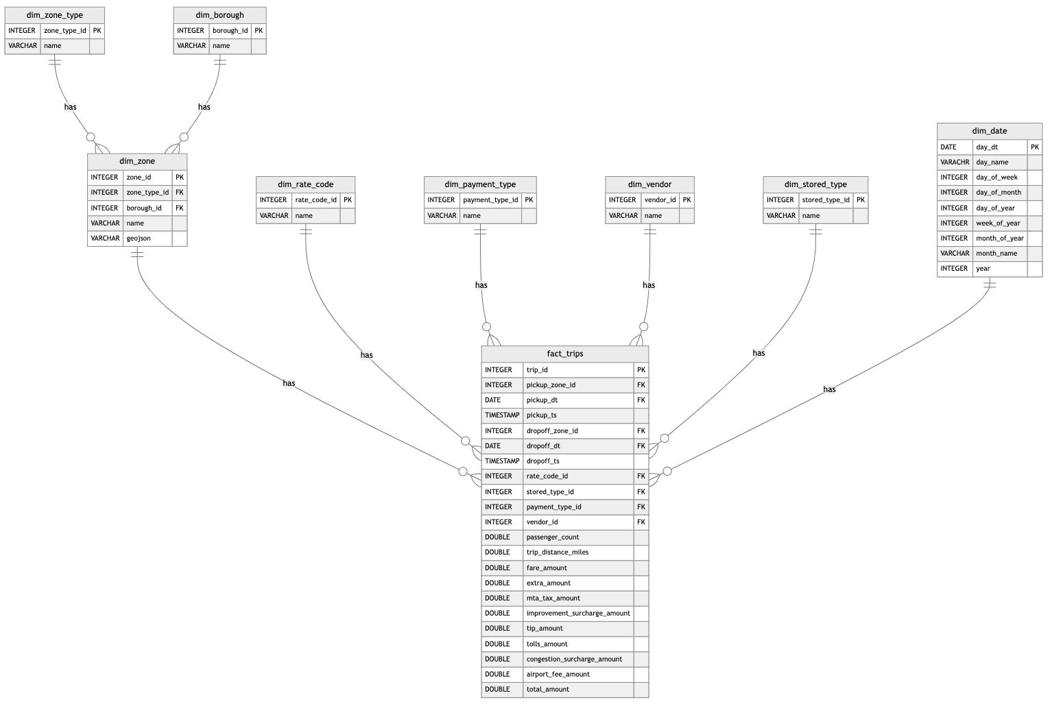
Target Data Model#
The target data model is derived from the original trip record data, with extracted dimension tables plus a new date hierarchy dimension. Also, the naming schema gets unified and cleaned up.
It is modeled as a so-called Snowflake Schema (check the Mermaid source):
Loading & Transforming the data#
The loading & transforming of the data is divided in multiple steps:
-
Generating the dimensional tables and values from the given dataset information
-
Generating a date hierarchy dimension
-
Loading and transforming the trip data
-
Replacing values with dimension references
-
Clean the column naming
-
Unify values
-
Generating the dimensional tables#
We use the given dataset information from the PDF file to manually create dimension tables and their values:
-- Install and load the spatial extension
INSTALL spatial;
LOAD spatial;

-- Create temporary table
CREATE TABLE tmp_service_zones AS (
    SELECT
        DISTINCT service_zone
    FROM
        'https://data.quacking.cloud/nyc-taxi-metadata/taxi_zones.csv'
    WHERE
        service_zone != 'N/A'
    ORDER BY
        service_zone
);

-- Create dim_zone_type table
CREATE TABLE dim_zone_type (
    zone_type_id INTEGER PRIMARY KEY,
    name VARCHAR
);

-- Insert dim_zone_type table
INSERT INTO dim_zone_type
SELECT
    -1 as zone_type_id,
    'N/A' as name
UNION ALL
SELECT
    (rowid + 1)::INTEGER as zone_type_id,
    service_zone as name
FROM
    tmp_service_zones
;

-- Drop table tmp_service_zones
DROP TABLE tmp_service_zones;

-- Create temporary table
CREATE TABLE tmp_borough AS (
    SELECT
        DISTINCT borough
    FROM
        'https://data.quacking.cloud/nyc-taxi-metadata/taxi_zones.csv'
    WHERE
        borough != 'Unknown'
    ORDER BY
        borough
);

-- Create dim_borough table
CREATE TABLE dim_borough (
    borough_id INTEGER PRIMARY KEY,
    name VARCHAR
);

-- Insert dim_borough table
INSERT INTO dim_borough
SELECT
    -1 as borough_id,
    'N/A' as name
UNION ALL
SELECT
    (rowid + 1)::INTEGER as borough_id,
    borough as name
FROM
    tmp_borough
;

-- Drop temporary table
DROP TABLE tmp_borough;

-- Create dim_zone table
CREATE TABLE dim_zone (
    zone_id INTEGER PRIMARY KEY,
    zone_type_id INTEGER,
    borough_id INTEGER,
    name VARCHAR,
    geojson VARCHAR,
    FOREIGN KEY (zone_type_id) REFERENCES dim_zone_type (zone_type_id),
    FOREIGN KEY (borough_id) REFERENCES dim_borough (borough_id)
);

-- Insert dim_zone table
INSERT INTO dim_zone
SELECT DISTINCT
    CASE
        WHEN csv.LocationID IS NOT NULL THEN csv.LocationID::INT
        ELSE raw.LocationID
    END AS zone_id,
    zt.zone_type_id,
    CASE
        WHEN b.borough_id IS NOT NULL THEN b.borough_id
        ELSE -1
    END AS borough_id,
    CASE
        WHEN csv.Zone IS NOT NULL THEN csv.Zone
        ELSE raw.zone
    END AS name,
    raw.geojson
FROM
    (
        SELECT
            LocationID,
            borough,
            zone,
            geojson
        FROM
            (
                SELECT
                    LocationID,
                    borough,
                    zone,
                    rank() OVER (PARTITION BY LocationID ORDER BY Shape_Leng) AS ranked,
                    ST_AsGeoJSON(ST_Transform(geom, 'ESRI:102718', 'EPSG:4326')) AS geojson
                FROM ST_Read('https://data.quacking.cloud/nyc-taxi-metadata/taxi_zones.shx')
            ) sub
        WHERE
            sub.ranked = 1
    ) raw
FULL OUTER JOIN
    (
        SELECT DISTINCT
            LocationID,
            Zone,
            service_zone
        FROM
            'https://data.quacking.cloud/nyc-taxi-metadata/taxi_zones.csv'
    ) csv
ON
    csv.LocationId = raw.LocationId
FULL OUTER JOIN
    dim_zone_type zt
ON
    csv.service_zone = zt.name
FULL OUTER JOIN
    dim_borough b
ON
    b.name = raw.borough
WHERE
    zone_id IS NOT NULL
ORDER BY
    zone_id
;

-- Create dim_rate_code table
CREATE TABLE dim_rate_code (
    rate_code_id INTEGER PRIMARY KEY,
    name VARCHAR
);

INSERT INTO dim_rate_code (rate_code_id, name) VALUES (1, 'Standard rate');
INSERT INTO dim_rate_code (rate_code_id, name) VALUES (2, 'JFK');
INSERT INTO dim_rate_code (rate_code_id, name) VALUES (3, 'Newark');
INSERT INTO dim_rate_code (rate_code_id, name) VALUES (4, 'Nassau or Westchester');
INSERT INTO dim_rate_code (rate_code_id, name) VALUES (5, 'Negotiated fare');
INSERT INTO dim_rate_code (rate_code_id, name) VALUES (6, 'Group ride');
INSERT INTO dim_rate_code (rate_code_id, name) VALUES (99, 'N/A');

-- Create dim_payment_type table
CREATE TABLE dim_payment_type (
    payment_type_id INTEGER PRIMARY KEY,
    name VARCHAR
);

INSERT INTO dim_payment_type (payment_type_id, name) VALUES (1, 'Credit card');
INSERT INTO dim_payment_type (payment_type_id, name) VALUES (2, 'Cash');
INSERT INTO dim_payment_type (payment_type_id, name) VALUES (3, 'No charge');
INSERT INTO dim_payment_type (payment_type_id, name) VALUES (4, 'Dispute');
INSERT INTO dim_payment_type (payment_type_id, name) VALUES (5, 'Unknown');
INSERT INTO dim_payment_type (payment_type_id, name) VALUES (6, 'Voided trip');

-- Create dim_vendor table
CREATE TABLE dim_vendor (
    vendor_id INTEGER PRIMARY KEY,
    name VARCHAR
);

INSERT INTO dim_vendor (vendor_id, name) VALUES (1, 'Creative Mobile Technologies');
INSERT INTO dim_vendor (vendor_id, name) VALUES (2, 'VeriFone Inc.');

-- Create dim_stored_type table
CREATE TABLE dim_stored_type (
    stored_type_id INTEGER PRIMARY KEY,
    name VARCHAR
);

INSERT INTO dim_stored_type (stored_type_id, name) VALUES (1, 'Store and forward trip');
INSERT INTO dim_stored_type (stored_type_id, name) VALUES (2, 'Not a store and forward trip');
Generating a date hierarchy dimension#
-- Create dim_date table
CREATE TABLE dim_date (
    day_dt DATE PRIMARY KEY,
    day_name VARCHAR,
    day_of_week INT,
    day_of_month INT,
    day_of_year INT,
    week_of_year INT,
    month_of_year INT,
    month_name VARCHAR,
    year INT
);

INSERT INTO dim_date
SELECT
    date_key AS day_dt,
    DAYNAME(date_key)::VARCHAR AS day_name,
    ISODOW(date_key)::INT AS day_of_week,
    DAYOFMONTH(date_key)::INT AS day_of_month,
    DAYOFYEAR(date_key)::INT AS day_of_year,
    WEEKOFYEAR(date_key)::INT AS week_of_year,
    MONTH(date_key)::INT AS month_of_year,
    MONTHNAME(date_key)::VARCHAR AS month_name,
    YEAR(date_key)::INT AS year
FROM
    (
        SELECT
            CAST(RANGE AS DATE) AS date_key
        FROM
            RANGE(DATE '2005-01-01', DATE '2030-12-31', INTERVAL 1 DAY)
    ) generate_date
;
Loading and transforming the trip data#
-- Create sequence for generating trip_ids
CREATE SEQUENCE trip_id_sequence START 1;

-- Create fact_trip table
CREATE TABLE fact_trip (
    trip_id INTEGER  DEFAULT nextval('trip_id_sequence') PRIMARY KEY,
    pickup_zone_id INTEGER,
    pickup_dt DATE,
    pickup_ts TIMESTAMP,
    dropoff_zone_id INTEGER,
    dropoff_dt DATE,
    dropoff_ts TIMESTAMP,
    rate_code_id INTEGER,
    stored_type_id INTEGER,
    payment_type_id INTEGER,
    vendor_id INTEGER,
    passenger_count DOUBLE,
    trip_distance_miles DOUBLE,
    fare_amount DOUBLE,
    extra_amount DOUBLE,
    mta_tax_amount DOUBLE,
    improvement_surcharge_amount DOUBLE,
    tip_amount DOUBLE,
    tolls_amount DOUBLE,
    congestion_surcharge_amount DOUBLE,
    airport_fee_amount DOUBLE,
    total_amount DOUBLE
);

-- Deactivating FK relationships for now, due to performance issues when inserting 3 million records
-- FOREIGN KEY (pickup_zone_id) REFERENCES dim_zone (zone_id),
-- FOREIGN KEY (dropoff_zone_id) REFERENCES dim_zone (zone_id),
-- FOREIGN KEY (pickup_dt) REFERENCES dim_date (day_dt),
-- FOREIGN KEY (dropoff_dt) REFERENCES dim_date (day_dt),
-- FOREIGN KEY (rate_code_id) REFERENCES dim_rate_code (rate_code_id),
-- FOREIGN KEY (stored_type_id) REFERENCES dim_stored_type (stored_type_id),
-- FOREIGN KEY (payment_type_id) REFERENCES dim_payment_type (payment_type_id),
-- FOREIGN KEY (vendor_id) REFERENCES dim_vendor (vendor_id)

-- Insert transformed fact data
INSERT INTO fact_trip
SELECT
    nextval('trip_id_sequence') AS trip_id,
    PULocationID::INT as pickup_zone_id,
    tpep_pickup_datetime::DATE as pickup_dt,
    tpep_pickup_datetime AS pickup_ts,
    DOLocationID::INT as dropoff_zone_id,
    tpep_dropoff_datetime::DATE as dropoff_dt,
    tpep_dropoff_datetime AS dropoff_ts,
    RatecodeID::INT AS rate_code_id,
    CASE
        WHEN store_and_fwd_flag = 'Y' THEN 1
        WHEN store_and_fwd_flag = 'N' THEN 2
    END AS stored_type_id,
    payment_type::INT AS payment_type_id,
    VendorID::INT AS vendor_id,
    passenger_count,
    trip_distance AS trip_distance_miles,
    fare_amount,
    extra AS extra_amount,
    mta_tax AS mta_tax_amount,
    improvement_surcharge AS improvement_surcharge_amount,
    tip_amount,
    tolls_amount,
    congestion_surcharge AS congestion_surcharge_amount,
    airport_fee AS airport_fee_amount,
    total_amount
FROM
    'https://data.quacking.cloud/nyc-taxi-data/yellow_tripdata_2023-01.parquet'
;
Data Analysis#
The following analyses are just examples on how you could analyze the data set. Feel free to think about your own questions for the dataset, and try to build queries yourselves!
Preparation#
DuckDB supports the SUMMARIZE command can help you understand the final data in the fact table before querying it. It launches a query that computes a number of aggregates over all columns, including min, max, avg, std and approx_unique:
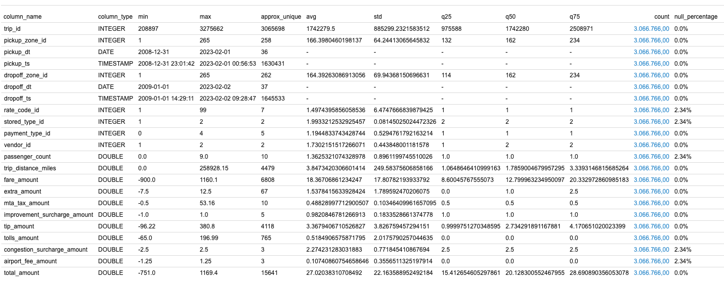
The output already shows some “interesting” things, such as pickup_dt being far in the past, e.g. 2008-12-31, and the dropoff_dt with similar values (2009-01-01).
Most utilized trip locations#
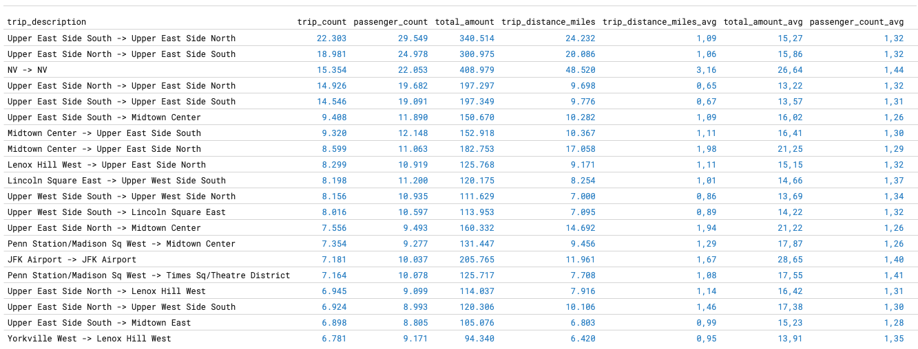
With this analysis, we want to have a look at the 20 most frequented trips from pickup zone to dropoff zone:
SELECT
    pz.name || ' -> ' || dz.name AS trip_description,
    count(DISTINCT ft.trip_id)::INT AS trip_count,
    sum(ft.passenger_count)::INT AS passenger_count,
    sum(ft.total_amount)::INT AS total_amount,
    sum(ft.trip_distance_miles)::INT AS trip_distance_miles,
    (sum(trip_distance_miles)/count(DISTINCT ft.trip_id))::DOUBLE AS trip_distance_miles_avg,
    (sum(ft.total_amount)/count(DISTINCT ft.trip_id))::DOUBLE AS total_amount_avg,
    (sum(ft.passenger_count)/count(DISTINCT ft.trip_id))::DOUBLE AS passenger_count_avg
FROM
    fact_trip ft
INNER JOIN
    dim_zone pz
ON
    pz.zone_id = ft.pickup_zone_id
INNER JOIN
    dim_zone dz
ON
    dz.zone_id = ft.dropoff_zone_id
GROUP BY
    trip_description
ORDER BY
    trip_count DESC
LIMIT 20;
On a M2 Mac Mini with 16GB RAM, aggregating the 3 million trips takes around 900ms. The result looks like the following:
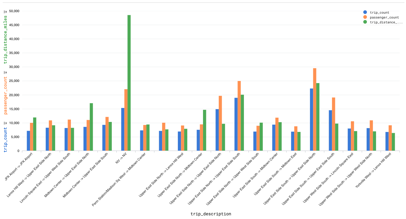
We can now also create a Y Bar chart showing the (total) trip count, passenger count and trip distance by top 20 most frequented trips:
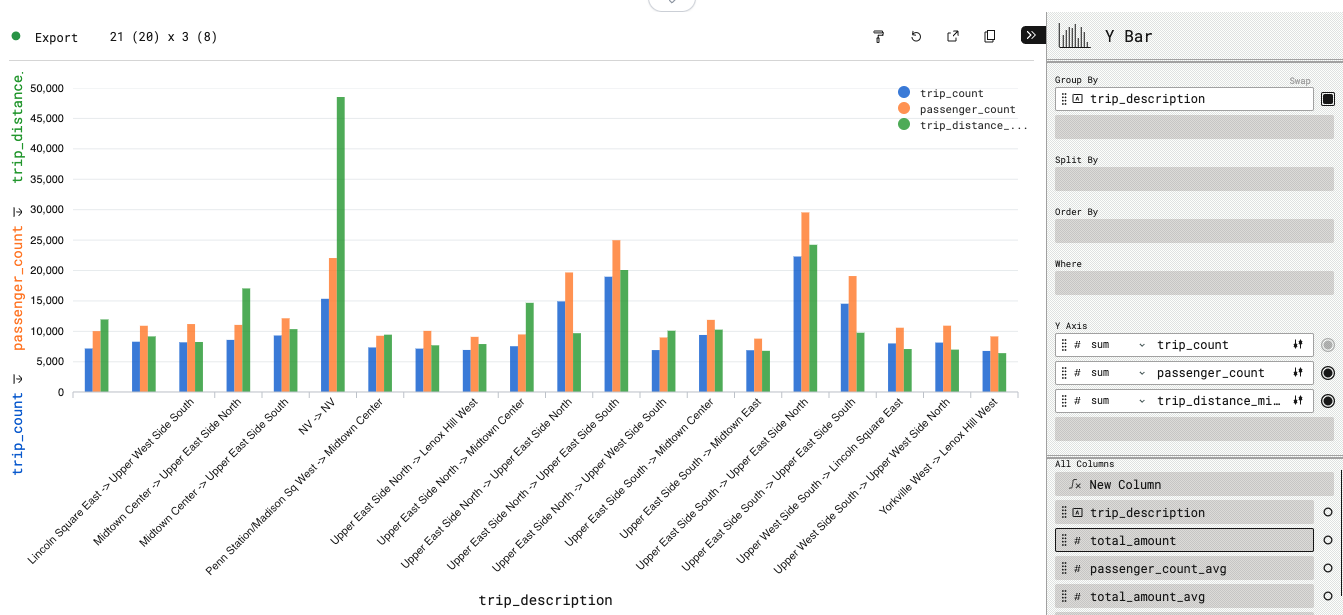
End result:
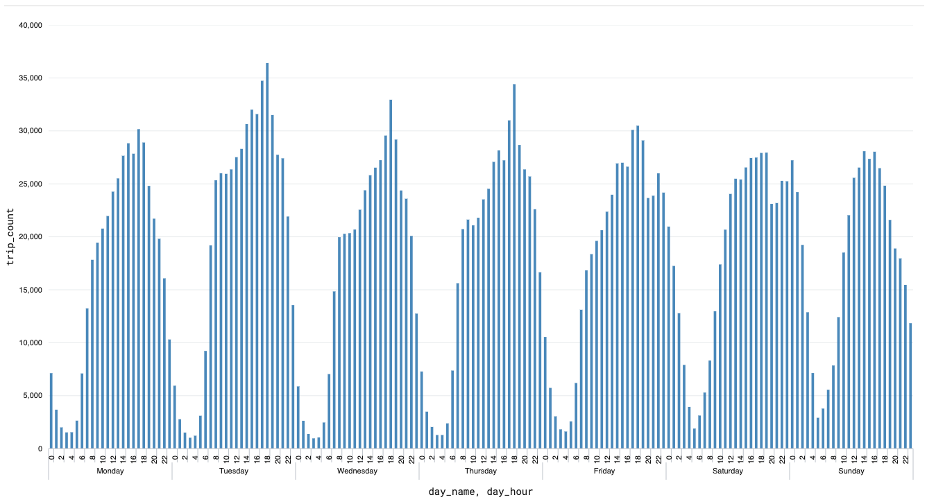
Trip frequency by weekday and time of day#
To inspect the traffic patterns, we want to analyze the trip frequency by weekday and time of day (aggregated on hourly level). Therefore, we make use of DuckDB’s advanced timestamp/time handling functions:
SELECT
    dd.day_name,
    dd.day_of_week,
    datepart('hour', time_bucket(INTERVAL '1 HOUR', ft.pickup_ts)) day_hour,
    count(DISTINCT ft.trip_id)::INT AS trip_count,
FROM
    fact_trip ft
INNER JOIN
    dim_date dd
ON
    dd.day_dt = ft.pickup_dt
GROUP BY
    dd.day_name,
    dd.day_of_week,
    day_hour
ORDER BY
    dd.day_of_week,
    day_hour;
Then, we can configure a Y Bar chart that can show us the number of trips by weekday and hour:
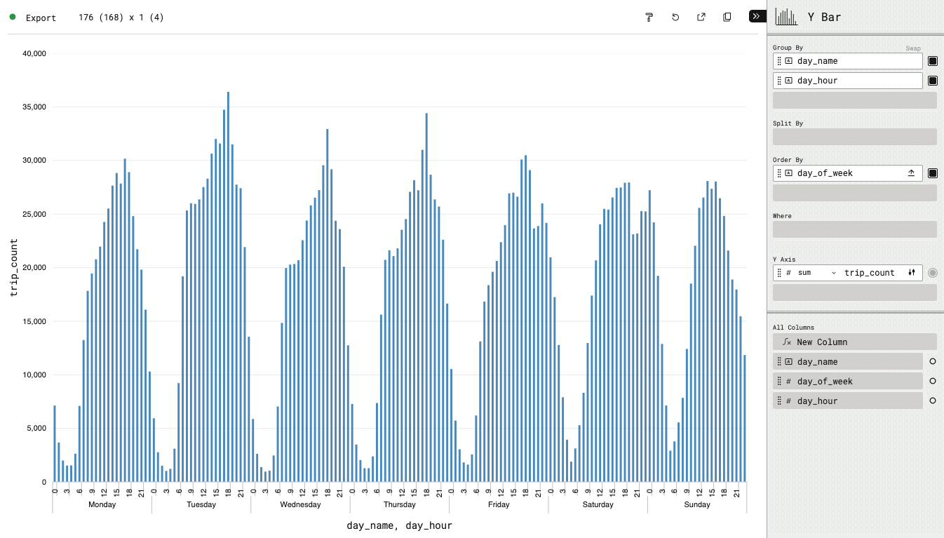
End result:
Sharing of Data Pipelines & Visualizations#
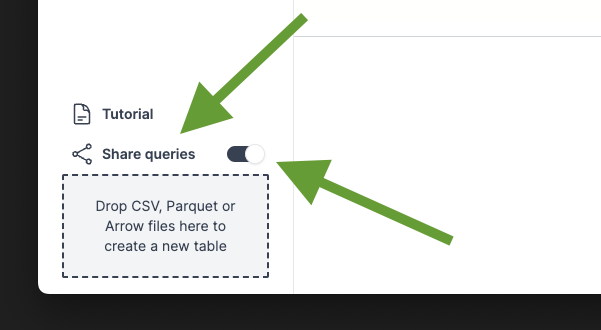
With the latest version of sql-workbench.com it’s possible to share both queries and the (customized) visualization of the last executed query. Therefore, you write your queries, run them to check whether they work, and then update the visualization configuration.
When you did that, you can then click on “Share queries” in the lower left corner of the SQL Workbench. The toggle will let you choose whether you want to copy the visualization configuration as well, or not.
If you want to run the complete pipeline to build our dimensional data model, you can click on the link below (this can take from 10 to 120 seconds depending on your machine and internet connection speed, as approximately 50MB of data will be downloaded):
Attaching remote databases#
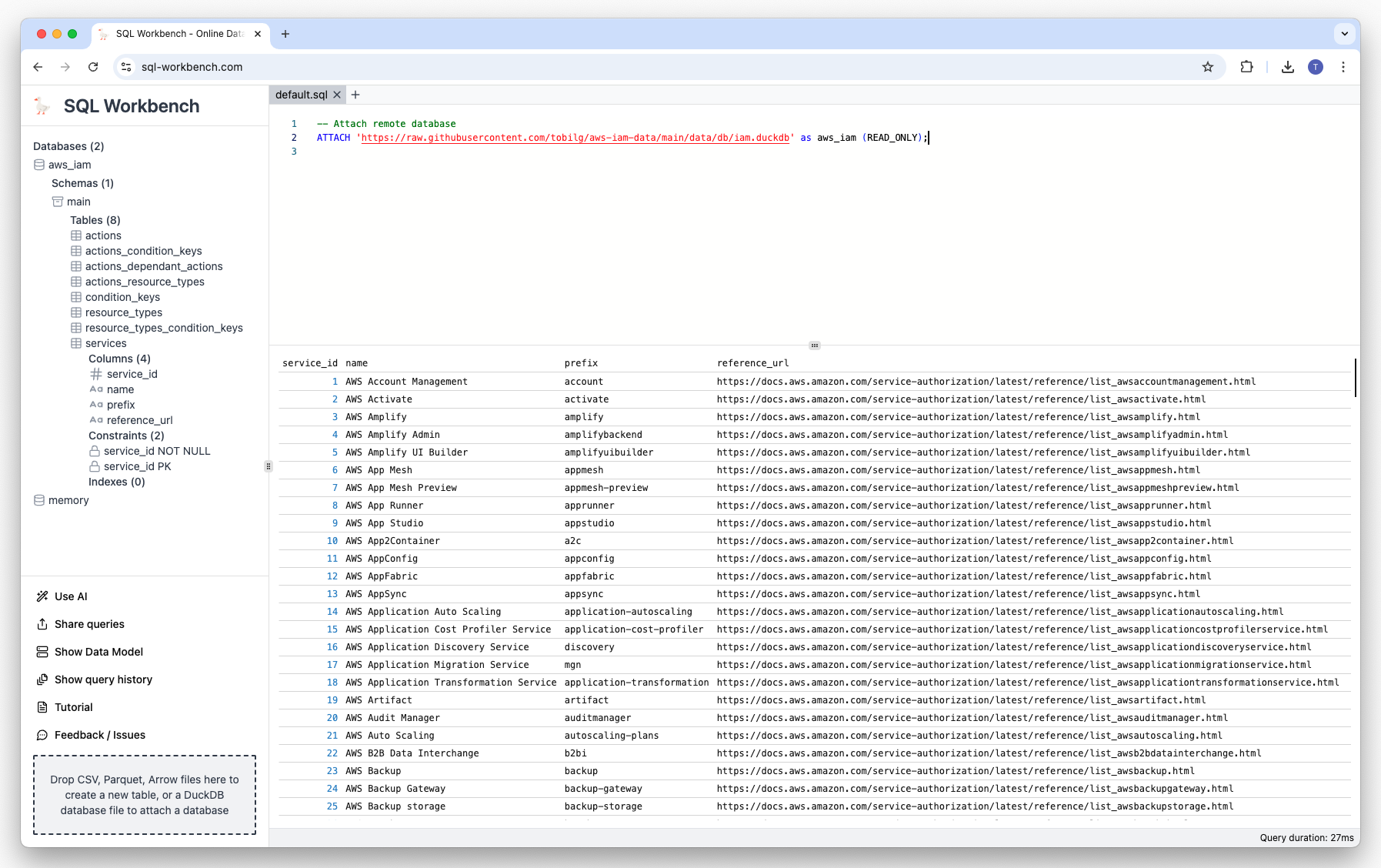
Since DuckDB v1.0.0, it is possible to attach a remote database via HTTPS or S3. As an example, you could use the below statements to load and query a remote dataset of AWS IAM data from GitHub:
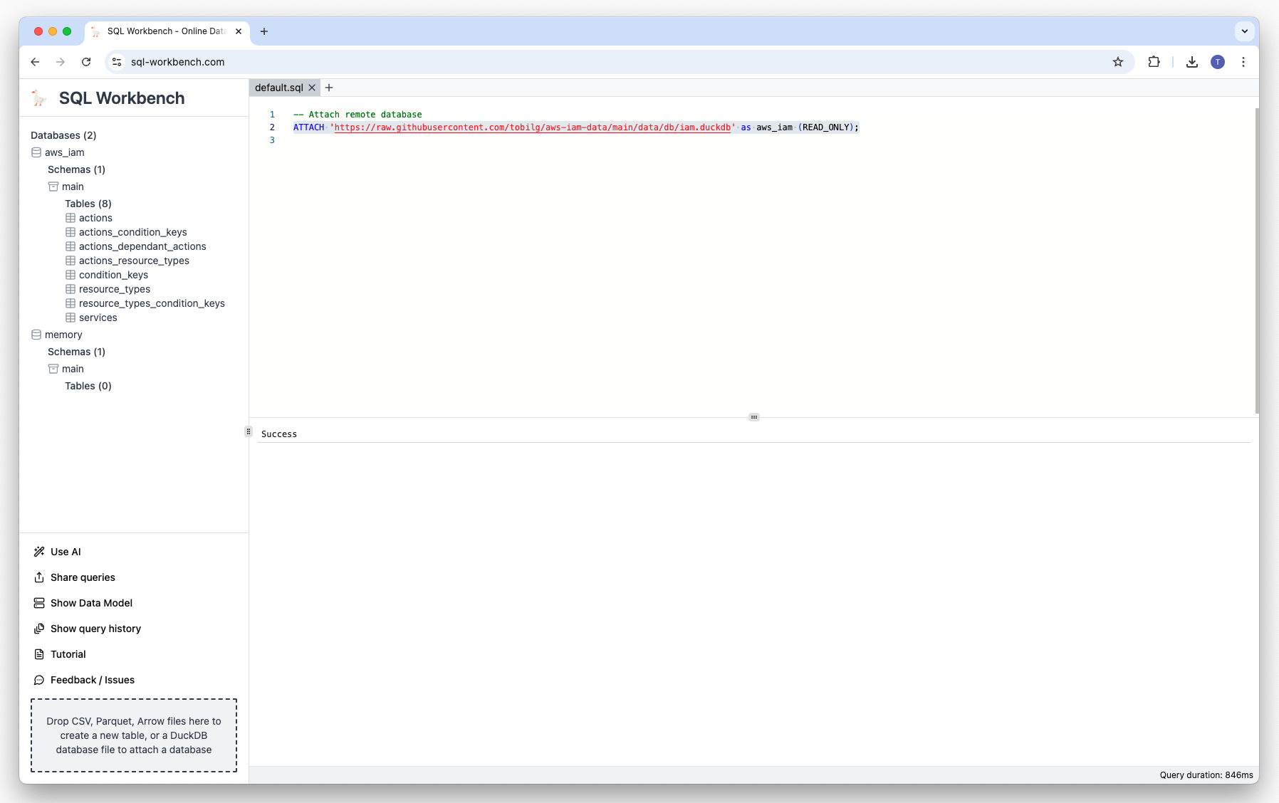
ATTACH 'https://raw.githubusercontent.com/tobilg/aws-iam-data/main/data/db/iam.duckdb' AS iam (READ_ONLY);

SELECT
  s.name as service_name,
  count(distinct a.name)::int action_cnt
FROM
  iam.services s
INNER JOIN
  iam.actions a ON s.service_id = a.service_id
GROUP BY ALL
ORDER BY action_cnt desc
LIMIT 25;
Click on the image below to execute the queries:
Conclusion#
With DuckDB-WASM and some common web frameworks, it’s pretty easy and fast to create custom data applications that can handle datasets in the size of millions of records.
Those applications are able to provide a very lightweight approach to working with different types of data (such as Parquet, Iceberg, Arrow, CSV, JSON or spatial data formats), whether locally or remote (via HTTP(S) of S3-compatible storage services), thanks to the versatile DuckDB engine.
Users can interactively work with the data, create data pipelines by using raw SQL, and iterate until the final desired state has been achieved. The generated data pipeline queries can easily be shared with simple links to sql-workbench.com, so that other collaborators can continue to iterate on the existing work, or even create new solutions with it.
Once a data pipeline has been finalized, it could for example be deployed to DuckDB instances running in own cloud accounts of the users. A great example would be running DuckDB in AWS Lambda, e.g. for repartitioning Parquet data in S3 nightly, or automatically running reports based on aggregation pipelines etc.
The possibilities are nearly endless, so I’m very curious what you all build with this great technology! Thanks for reading this length article, I’m happy to answer any questions in the comments.